Note
Click here to download the full example code
Sampling along tracks
The pygmt.grdtrack function samples a raster grid’s value along specified
points. We will need to input a 2D raster to grid which can be an
xarray.DataArray. The points parameter can be a pandas.DataFrame table where
the first two columns are x and y (or longitude and latitude). Note also that there is a
newcolname parameter that will be used to name the new column of values we sampled
from the grid.
Alternatively, we can provide a NetCDF file path to grid. An ASCII file path can
also be accepted for points, but an outfile parameter will then need to be set
to name the resulting output ASCII file.
Out:
gmtwhich [NOTICE]: Remote data courtesy of GMT data server OCEANIA [https://oceania.generic-mapping-tools.org]
gmtwhich [NOTICE]: Earth Relief at 1x1 arc degrees from Gaussian Cartesian filtering (111 km fullwidth) of SRTM15+V2.1 [Tozer et al., 2019].
gmtwhich [NOTICE]:   -> Download grid file [115K]: earth_relief_01d_p.grd
gmtwhich [NOTICE]:   -> Download cache file: @ridge.txt

<IPython.core.display.Image object>
import pygmt
# Load sample grid and point datasets
grid = pygmt.datasets.load_earth_relief()
points = pygmt.datasets.load_ocean_ridge_points()
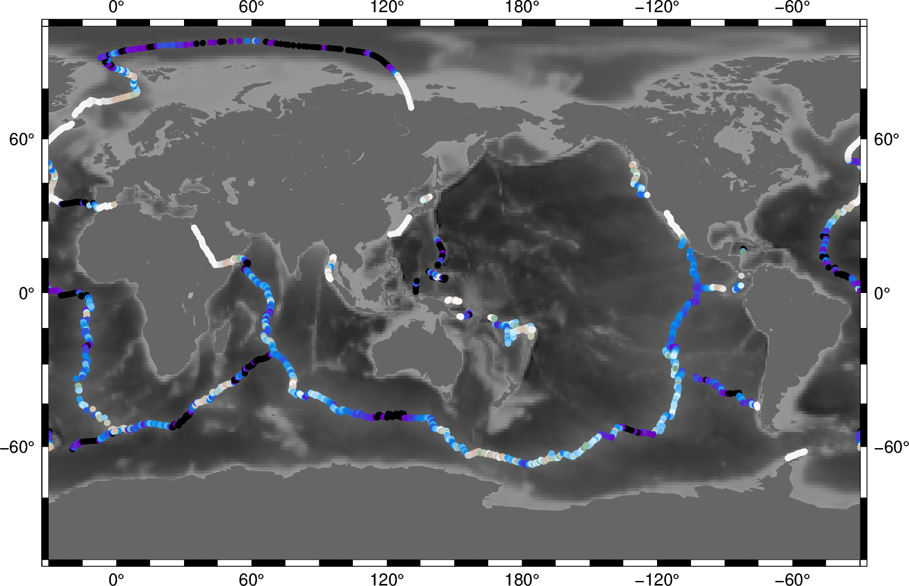
# Sample the bathymetry along the world's ocean ridges at specified track points
track = pygmt.grdtrack(points=points, grid=grid, newcolname="bathymetry")
fig = pygmt.Figure()
# Plot the earth relief grid on Cylindrical Stereographic projection, masking land areas
fig.basemap(region="g", frame=True, projection="Cyl_stere/150/-20/8i")
fig.grdimage(grid=grid, cmap="gray")
fig.coast(land="#666666")
# Plot using circles (c) of 0.15cm, the sampled bathymetry points
# Points are colored using elevation values (normalized for visual purposes)
fig.plot(
x=track.longitude,
y=track.latitude,
style="c0.15c",
cmap="terra",
color=(track.bathymetry - track.bathymetry.mean()) / track.bathymetry.std(),
)
fig.show()
Total running time of the script: ( 0 minutes 3.020 seconds)